WHY?

Representing bilinear relationship of two inputs is expensive. MLB efficiently reduced the number of parameters by substituting bilinear operation with Hadamard product operation. This paper extends this idea to capture bilinear attention between two multi-channel inputs.

WHAT?

Using the low-rank bilinear pooling, attention on visual inputs given a question vector can be calculated efficiently. This can be generalized to represent a bilinear model for two multi-channel inputs. While $\mathbf{f}_k'$ indicates kth element of intermediate representation,

$$\mathbf{f}_k' = (\mathbf{X}^T\mathbf{U}')^T_k\mathcal{K}(\mathbf{Y}^T\mathbf{V}')_k\\ = \sum_{i=1}^{\rho}\sum_{j=1}^{\phi}\mathcal{A}_{ij}(\mathbf{X}^T_i\mathbf{U}_k')(\mathbf{V}'_k^T\mathbf{Y}_j) = \sum_{i=1}^{\rho}\sum_{j=1}^{\phi}\mathcal{A}_{ij}\mathbf{X}_i^T(\mathbf{U}_k'\mathbf{V}_k'^T)\mathbf{Y}_j\\ \mathbf{f} = \mathbf{P}^T\mathbf{f}'\\ = BAN(\mathbf{X}, \mathbf{Y}; \mathcal{A})$$

Attention between two input channels can be calculated similarly as in MLB.

$$\mathcal{A}_g = softmax(((1\cdot\mathbf{p}_g^T)\circ \mathbf{X}^T\mathbf{U})\mathbf{V}^T\mathbf{Y})$$

BAN reflects the linear projection of multiple co-attention.

Low-rank bilinear pooling allowed efficient calculation of multiple glimpses of attention distribution given a single reference vector. BAN generalized this idea for two multi-channel inputs.

$$ \mathbf{f’}_k=(\mathbf{X}^T\mathbf{U’})^T_K\mathcal{A}(\mathbf{Y}^T\mathbf{V}’)_k\

Reading and writing in DNC are implemented with differentiable attention mechanism.

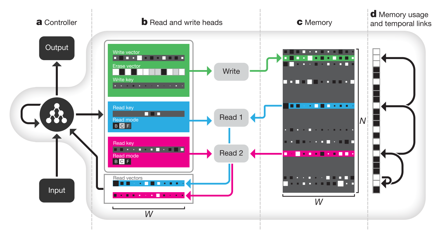
The controller of DNC is an variant of LSTM architecture that takes an input vector($x_t$) and a set of read vectors($r_{t-1}^1,...,r_{t-1}^R$) as input(concatenated). Concatenated input and hidden vectors from both previous timestep($h_{t-1}^l$) and from previous layer($h_t^{l-1}$) are concatenated again to be used as input for LSTM to produce next hidden vector($h_t^l$). Hidden vectors from all layers at a timestep are concatenated to emit an output vector($\upsilon_t$) and an interface vector($\xi_t$). The output vector($y_t$) is the sum of $\upsilon_t$ and read vectors of the current timestep.

$$v_t = W_y[h_t^1;...;h_t^L]\\ \xi_t = W_{\xi}[h_t^1;...;h_t^L]\\ y_t = \upsilon_t + W_t[r_t^1;...;r_t^R]$$

THe interface vectors are consists of many vectors that interacts with memory: R read keys($\mathbf{k}_t^{r,i}\in R^W$), read strengths($\beta_t^{r,i}$), write key($\mathbf{k}_t^w\in R^W$), write strength($\beta_t^w$), erase vector($\mathbf{e}_t\in R^W$), write vector($\mathbf{v}_t\in R^W$), R free gates($f_t^i$), the allocation gate($g_t^a$), the write gate($g_t^w$) and R read modes(\mathbf{\pi}_t^i).

$$\mathbf{\xi}_t = [\mathbf{k}_t^{r,1};...;\mathbf{k}_t^{r,R};\beta_t^{r,1};...;\beta_t^{r,R};\mathbf{k}_t^w;\beta_t^w;\mathbf{e}_t;\mathbf{v}_t;f_t^1;...;f_t^R;g_t^a;g_t^w;\mathbf{\pi}_t^1;...;\mathbf{\pi}_t^R]$$

Read vectors are computed with read weights on memory. Memory matrix are updated with write weights, write vector and erase vector.

$$\mathbf{r}_t^i = M_t^T\mathbf{w}_t^{r,i}\\ M_t = M_{t-1}\odot(E-\mathbf{w}^w_t\mathbf{e}_t^T)+\mathbf{w}^w_t\mathbf{v}_t^T$$

Memory are addressed with content-based addressing and dynamic memory allocation. Contesnt-based addressing is basically the same as attention mechanism. Dynamic memory allocation is designed to clear memory as analogous to free list memory allocation scheme.

So?

DNC showed good result on bAbI task, and Graph tasks.

Graves, Alex, et al. “Hybrid computing using a neural network with dynamic external memory.” Nature 538.7626 (2016): 471.