WHY?

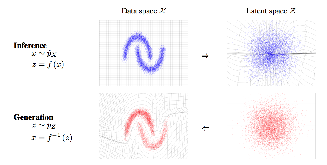The motivation is almost the same as that of NICE. This papaer suggest more elaborate transformation to represent complex data.

WHAT?

NICE suggested coupling layers with tractable Jacobian matrix. This paper suggest flexible bijective function while keeping the property of coupling layers. Affine coupling layers scale and translate the x, its Jacobian is easy to compute and invertible. In this paper, s and t are used as rectified convolution layer. 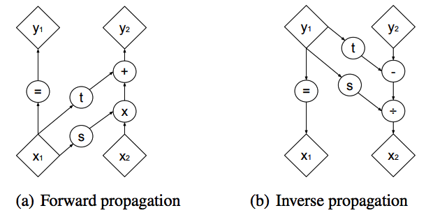$y_{1:d} = x_{1:d}\\ y_{d+1:D} = x_{d+1:D}\odot \exp(s(d_{x:d})) + t(x_{1:d})\\ \frac{\partial y}{\partial x^T} = \left[\begin{array}{cc} I_d & 0\\\frac{\partial y_{d+1:D}}{\partial x^T_{1:d}} & diag(\exp[s(x_{1:d})]) \end{array} \right]\\ x_{1:d} = y_{1:d} \\ x_{d+1:D} = (y_{d+1:D} - t(y_{1:d}))\odot \exp(-s(y_{1:d}))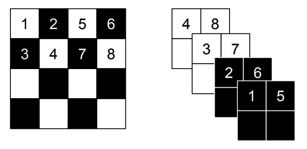$ This paper suggested two ways for partition. First is spatial checkerboard patterns and second is channel-wise masking (above). 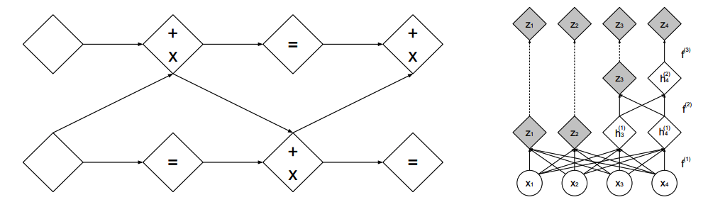To build up this components into a multiscale architecture, squeezing operation is used to divide a channel into four (above). A scale in architecture consists of three coupling layers with checkerboard masks, squeezing operation and three more coupling layers with alternating channel-wise masking. $h^{(0)} = x\\ (z^{(i+1)}, h^{(i+1)}) = f^{(i+1)}(h^{(i)})\\ z^{(L)} = f^{(L)}(h^{(L-1)})\\ z = (z^{(1)}), ..., z^{(L)}$ Batch normalization is use whose Jacobian matrix is also tractable. $\left(\prod)_i(\tilde{\sigma}_i^2 + \epsilon)\right)^{-\frac{1}{2}}\\$

So?

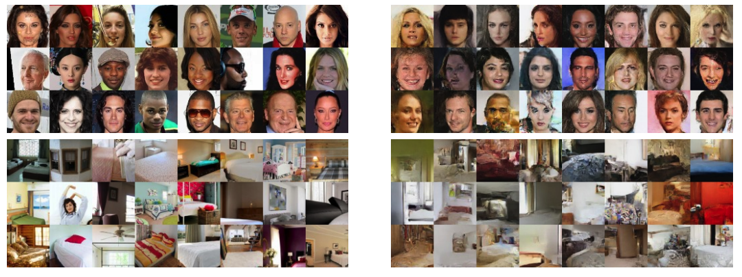Real NVP showed competitive performance in generation in CIFAR10, Imagenet, CelebA, and LSUN in terms of quality and log likelihood.

Critic

Are prior distributions trainable? I wonder if diverse form of priors affect the quality of sample.

Dinh, Laurent, Jascha Sohl-Dickstein, and Samy Bengio. “Density estimation using Real NVP.” arXiv preprint arXiv:1605.08803 (2016).